Laboratory setup#

Laboratory set-up for non-linear spectroscopy

This class controls calculations of non-linear optical spectra, and other experiments in which laboratory setting needs to be controlled. Examples are pulse polarization setting, pulse shapes and spectra in non-linear spectroscopy.

Class Details#

class quantarhei.spectroscopy.labsetup.LabSetup(nopulses: int = 3)[source]#

Bases: object

Laboratory set-up for non-linear spectroscopy

Class representing laboratory setup for non-linear spectroscopic experiments. It holds information about pulse shapes and polarizations.

Pulses can be set in time- and/or frequency-domain. Consistency between the domains is not checked nor enforced. Consistent conversion between domains is provided by convenience routines [TO BE IMPLEMENTED]

Parameters:: nopulses (int) – Number of pulses in the experiment. Default is 3.

property number_of_pulses: Any#

reset_pulse_shape() → None[source]#: Recalculates the pulse shapes

set_pulse_shapes(axis: Any, params: Any) → None[source]#

Sets the pulse properties

Pulse shapes or spectra are set in this routine. If axis is of TimeAxis type, the parameters are understood as time domain, if axis is of FrequencyAxis type, they are understood as frequency domain.

Parameters:

axis (TimeAxis or FrequencyAxis) – Quantarhei time axis object, which specifies the values for which pulse properties are defined. If TimeAxis is specified, the parameters are understood as time domain, if FrequencyAxis is specified, they are understood as frequency domain.
params (dictionary) –
Dictionary of pulse parameters. The parameters are the following: ptype is the pulse type with possible values Gaussian and numeric. Time domain pulses are specified with their center at t = 0.

Gaussian pulse has further parameters amplitude, FWHM, and frequency with obvious meanings. FWHM is speficied in fs, frequency is specified in energy units, while amplitude is in units of [energy]/[transition dipole moment]. The formula for the lineshape is

\[\rm{shape}(\omega) = \frac{2}{\Delta}\sqrt{\frac{\ln(2)}{\pi}} \exp\left\{-\frac{4\ln(2)\omega^2}{\Delta^2}\right\}\]

The same formulae are used for time- and frequency domain definitions. For time domain, \(t\) should be used in stead of \(\omega\).

numeric pulse is specified by a second parameters function which should be of DFunction type and specifies line shape around zero frequency.

Examples

>>> import quantarhei as qr
>>> import matplotlib.pyplot as plt
>>> lab = LabSetup()
...
>>> # Time axis around 0
>>> time = qr.TimeAxis(-500.0, 1000, 1.0, atype="complete")

Gaussian pulse shape in time domain

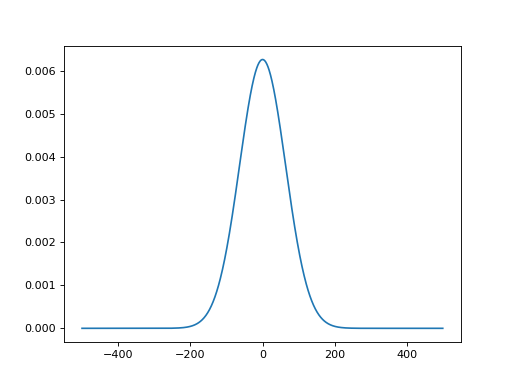
>>> pulse2 = dict(ptype="Gaussian", FWHM=150, amplitude=1.0)
>>> params = (pulse2, pulse2, pulse2)
>>> lab.set_pulse_arrival_times([0.0, 0.0, 0.0])
>>> lab.set_pulse_phases([0.0, 0.0, 0.0])  # these settings are compulsory
>>> lab.set_pulse_shapes(time, params)

Testing the pulse shape

>>> dfc = lab.get_pulse_envelop(1, time.data)
>>> pl = plt.plot(time.data, dfc)
>>> plt.show()

(Source code, png, hires.png, pdf)

numeric pulse shape in time domain

>>> # We take the DFunction for creation of `numeric`ly defined
>>> # pulse shape from the previous example
>>> pls = lab.pulse_t[2]
>>> # new lab object
>>> lab2 = LabSetup()

>>> pulse1 = dict(ptype="numeric", function=pls)
>>> params = (pulse1, pulse1, pulse1)
>>> lab2.set_pulse_arrival_times([0.0, 0.0, 0.0])
>>> lab2.set_pulse_phases([0.0, 0.0, 0.0])
>>> lab2.set_pulse_shapes(time, params)

Testing the pulse shape

>>> dfc = lab2.get_pulse_envelop(1, time.data)
>>> pl = plt.plot(time.data, dfc)
>>> plt.show() # we skip output here

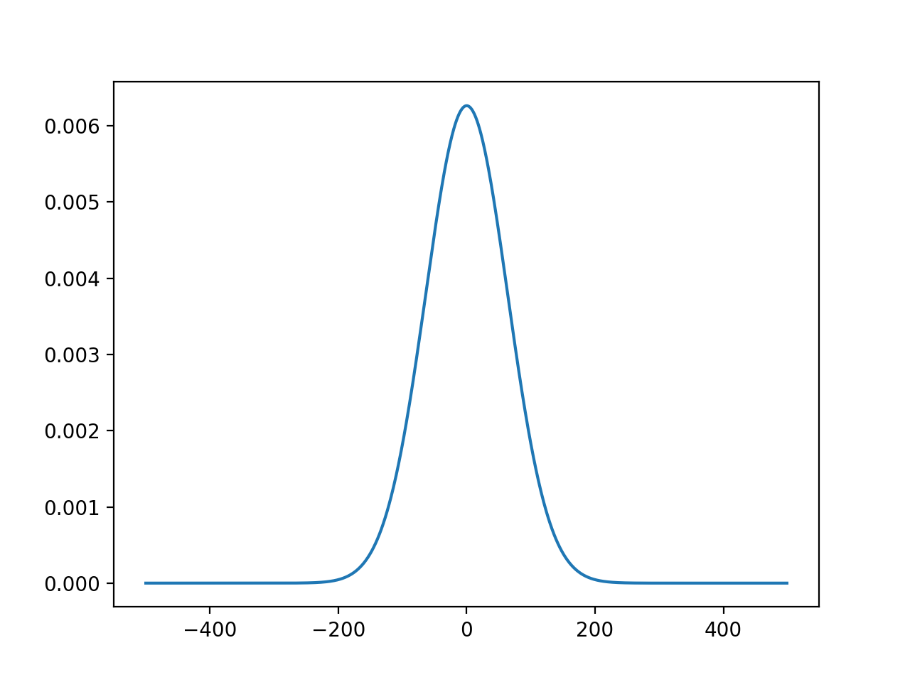
Gaussian pulse shape in frequency domain

>>> lab = LabSetup()
>>> # FrequencyAxis around 0
>>> freq = qr.FrequencyAxis(-2500, 1000, 5.0)
...
>>> pulse2 = dict(ptype="Gaussian", FWHM=800, amplitude=1.0)
>>> params = (pulse2, pulse2, pulse2)
>>> lab.set_pulse_arrival_times([0.0, 0.0, 0.0])
>>> lab.set_pulse_phases([0.0, 0.0, 0.0])
>>> lab.set_pulse_shapes(freq, params)

Testing the pulse shape

>>> # getting differnt frequency axis
>>> freq2 = qr.FrequencyAxis(-1003, 100, 20.0)
>>> # and reading spectrum at two different sets of points
>>> dfc1 = lab.get_pulse_spectrum(1, freq.data)
>>> dfc2 = lab.get_pulse_spectrum(1, freq2.data)
>>> pl1 = plt.plot(freq.data, dfc1)
>>> pl2 = plt.plot(freq2.data, fdc2)
>>> plt.show()

We plot in two different sets of points.

(Source code)

numeric pulse shape in frequency domain

>>> # We take the DFunction for creation of `numeric`ly defined
>>> # pulse shape from the previous example
>>> pls = lab.pulse_f[2]
>>> # new lab object
>>> lab2 = LabSetup()

>>> pulse1 = dict(ptype="numeric", function=pls)
>>> params = (pulse1, pulse1, pulse1)
>>> lab2.set_pulse_arrival_times([0.0, 0.0, 0.0])
>>> lab2.set_pulse_phases([0.0, 0.0, 0.0])
>>> lab2.set_pulse_shapes(freq, params)

Testing the pulse shape

>>> dfc = lab2.get_pulse_envelop(1, freq.data)
>>> pl = plt.plot(freq.data, dfc)
>>> plt.show() # we skip output here

Situations in which Exceptions are thrown

>>> pulse3 = dict(ptype="other", FWHM=10, amplitude=1.0)
>>> params = (pulse3, pulse3, pulse3)
>>> lab.set_pulse_shapes(time, params)
Traceback (most recent call last):
    ...
quantarhei.exceptions.QuantarheiError: Unknown pulse type

>>> params = (pulse2, pulse2)
>>> lab.set_pulse_shapes(time, params)
Traceback (most recent call last):
    ...
quantarhei.exceptions.QuantarheiError: set_pulses requires 3 parameter sets

>>> params = (pulse2, pulse2)
>>> lab.set_pulse_shapes(time.data, params)
Traceback (most recent call last):
    ...
quantarhei.exceptions.QuantarheiError: Wrong axis paramater

>>> time = qr.TimeAxis(0.0, 1000, 1.0)
>>> lab.set_pulse_shapes(time, params)
Traceback (most recent call last):
    ...
quantarhei.exceptions.QuantarheiError: TimeAxis has to be of 'complete' type use atype='complete' as a parameter of TimeAxis

set_pulse_polarizations(pulse_polarizations: Any = ((1.0, 0.0, 0.0), (1.0, 0.0, 0.0), (1.0, 0.0, 0.0)), detection_polarization: Any = (1.0, 0.0, 0.0)) → None[source]#

Sets polarizations of the experimental pulses

Parameters:

pulse_polarization (tuple like) – Contains three vectors of polarization of the three pulses of the experiment. Currently we assume three pulse experiment per default.
detection_polarization (array) – Vector of detection polarization

Examples

>>> import quantarhei as qr
>>> lab = LabSetup()
>>> lab.set_pulse_polarizations(pulse_polarizations=(qr.utils.vectors.X,
...                                            qr.utils.vectors.Y,
...                                            qr.utils.vectors.Z))
>>> print(lab.e[0,:])
[ 1.  0.  0.]
>>> print(lab.e[3,:])
[ 1.  0.  0.]
>>> print(lab.e[2,:])
[ 0.  0.  1.]

>>> lab.set_pulse_polarizations(pulse_polarizations=(qr.utils.vectors.X,
...                                            qr.utils.vectors.Y))
Traceback (most recent call last):
    ...
quantarhei.exceptions.QuantarheiError: pulse_polarizations requires 3 values

get_pulse_polarizations() → list[Any][source]#

Returns polarizations of the laser pulses

Examples

>>> import quantarhei as qr
>>> lab = LabSetup()
>>> lab.set_pulse_polarizations(pulse_polarizations=(qr.utils.vectors.X,
...                                            qr.utils.vectors.Y,
...                                            qr.utils.vectors.Z))
>>> pols = lab.get_pulse_polarizations()
>>> print(len(pols))
3

get_detection_polarization() → Any[source]#

Returns detection polarizations

Examples

>>> import quantarhei as qr
>>> lab = LabSetup()
>>> lab.set_pulse_polarizations(pulse_polarizations=(qr.utils.vectors.X,
...                                            qr.utils.vectors.Y,
...                                            qr.utils.vectors.Z))
>>> detpol = lab.get_detection_polarization()
>>> print(detpol)
[ 1.  0.  0.]

convert_to_time() → None[source]#

Converts pulse information from frequency domain to time domain

Examples

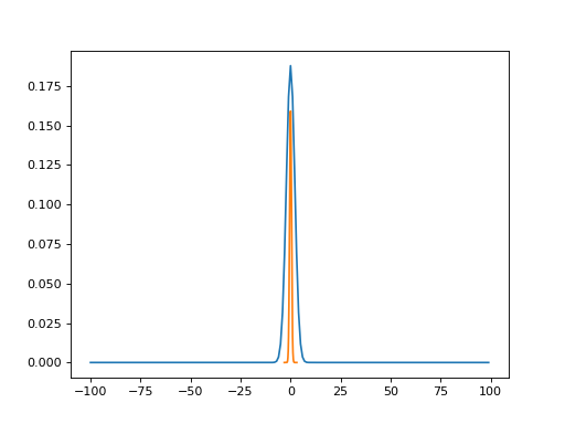
>>> import quantarhei as qr
>>> import matplotlib.pyplot as plt
>>> lab = LabSetup()
>>> freq = qr.FrequencyAxis(-100, 200, 1.0) # atype="complete" is default
>>> pulse = dict(ptype="Gaussian", FWHM=20, amplitude=1.0)
>>> params = (pulse, pulse, pulse)
>>> lab.set_pulse_arrival_times([0.0, 0.0, 0.0])
>>> lab.set_pulse_phases([0.0, 0.0, 0.0])
>>> lab.set_pulse_shapes(freq, params)
>>> lab.convert_to_time()
>>> # plot the original and the FT pulses
>>> pls_1f = lab.pulse_f[1]
>>> p1 = plt.plot(pls_1f.axis.data, pls_1f.data)
>>> pls_1t = lab.pulse_t[1]
>>> p2 = plt.plot(pls_1t.axis.data, pls_1t.data)
>>> plt.show()

(Source code, png, hires.png, pdf)

Now we compare back and forth Fourier transform with the original

>>> import quantarhei as qr
>>> import numpy
>>> lab = LabSetup()
>>> freq = qr.FrequencyAxis(-100,200,1.0) # atype="complete" is default
>>> pulse = dict(ptype="Gaussian", FWHM=20, amplitude=1.0)
>>> params = (pulse, pulse, pulse)
>>> lab.set_pulse_arrival_times([0.0, 0.0, 0.0])
>>> lab.set_pulse_phases([0.0, 0.0, 0.0])
>>> lab.set_pulse_shapes(freq, params)
>>> freq_vals_1 = lab.get_pulse_spectrum(2, freq.data)
>>> lab.convert_to_time()

Here we override the original frequency domain definition

>>> lab.convert_to_frequency()
>>> freq_vals_2 = lab.get_pulse_spectrum(2, freq.data)
>>> numpy.allclose(freq_vals_2, freq_vals_1)
True

and now the other way round

>>> import quantarhei as qr
>>> import numpy
>>> lab = LabSetup()
>>> time = qr.TimeAxis(-100,200,1.0, atype="complete")
>>> pulse = dict(ptype="Gaussian", FWHM=20, amplitude=1.0)
>>> params = (pulse, pulse, pulse)
>>> lab.set_pulse_arrival_times([0.0, 0.0, 0.0])
>>> lab.set_pulse_phases([0.0, 0.0, 0.0])
>>> lab.set_pulse_shapes(time, params)
>>> time_vals_1 = lab.get_pulse_envelop(2, time.data)
>>> lab.convert_to_frequency()

Here we override the original time domain definition

>>> lab.convert_to_time()
>>> time_vals_2 = lab.get_pulse_envelop(2, freq.data)
>>> numpy.allclose(time_vals_2, time_vals_1)
True

Situation in which excetions are thrown

>>> lab = LabSetup()
>>> lab.convert_to_time()
Traceback (most recent call last):
    ...
quantarhei.exceptions.QuantarheiError: Cannot convert to time domain: frequency domain not set

convert_to_frequency() → None[source]#

Converts pulse information from time domain to frequency domain

Examples

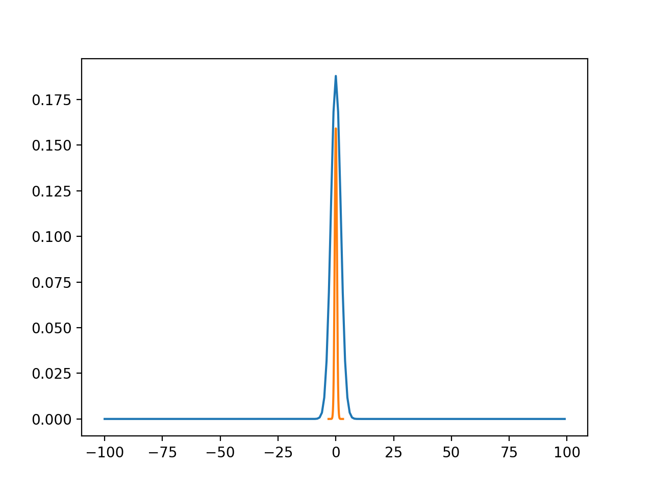
>>> import quantarhei as qr
>>> lab = LabSetup()
>>> time = qr.TimeAxis(-100,200,1.0, atype="complete")
>>> pulse = dict(ptype="Gaussian", FWHM=20, amplitude=1.0)
>>> params = (pulse, pulse, pulse)
>>> lab.set_pulse_arrival_times([0.0, 0.0, 0.0])
>>> lab.set_pulse_phases([0.0, 0.0, 0.0])
>>> lab.set_pulse_shapes(time, params)
>>> lab.convert_to_frequency()
>>> # plot the original and the FT pulses
>>> pls_1f = lab.pulse_f[1]
>>> plt.plot(pls_1f.axis.data, pls_1f.data)
>>> pls_1t = lab.pulse_t[1]
>>> plt.plot(pls_1t.axis.data, pls_1t.data)
>>> plt.show()

(Source code, png, hires.png, pdf)

Situation in which excetions are thrown

>>> lab = LabSetup()
>>> lab.convert_to_frequency()
Traceback (most recent call last):
    ...
quantarhei.exceptions.QuantarheiError: Cannot convert to frequency domain: time domain not set

get_pulse_envelop(k: int, t: Any) → Any[source]#

Returns a numpy array with the pulse time-domain envelope

Parameters:

k (int) – Index of the pulse to be returned
t (array like) – Array of time points at which the pulse is returned

Examples

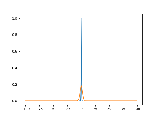
>>> import quantarhei as qr
>>> lab = LabSetup()
>>> time = qr.TimeAxis(-100, 200, 1.0, atype="complete")
>>> pulse2 = dict(ptype="Gaussian", FWHM=30.0, amplitude=1.0)
>>> params = (pulse2, pulse2, pulse2)
>>> lab.set_pulse_arrival_times([0.0, 0.0, 0.0])
>>> lab.set_pulse_phases([0.0, 0.0, 0.0])
>>> lab.set_pulse_shapes(time, params)
>>> dfc = lab.get_pulse_envelop(1, [-50.0, -30.0, 2.0, 30.0])
>>> print(dfc)
[  1.41569209e-05   1.95716100e-03   3.09310662e-02   1.95716100e-03]

import quantarhei as qr
import matplotlib.pyplot as plt

lab = qr.LabSetup()
time = qr.TimeAxis(-500.0, 1000, 1.0, atype="complete")
pulse2 = dict(ptype="Gaussian", FWHM=150.0, amplitude=1.0)
params = (pulse2, pulse2, pulse2)
lab.set_pulse_arrival_times([0.0, 0.0, 0.0])
lab.set_pulse_phases([0.0, 0.0, 0.0])
lab.set_pulse_shapes(time, params)

pls = lab.pulse_t[2]
lab2 = qr.LabSetup()

pulse1 = dict(ptype="numeric", function=pls)
params = (pulse1, pulse1, pulse1)
lab2.set_pulse_arrival_times([0.0, 0.0, 0.0])
lab2.set_pulse_phases([0.0, 0.0, 0.0])
lab2.set_pulse_shapes(time, params)

dfc = lab2.get_pulse_envelop(1, time.data)
pl = plt.plot(time.data, dfc)
plt.show()

(Source code, png, hires.png, pdf)

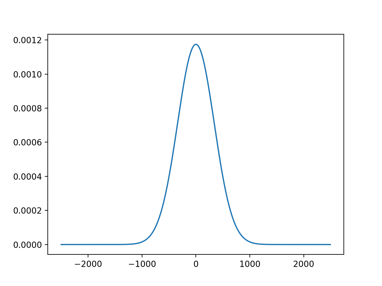
get_pulse_spectrum(k: int, omega: Any) → Any[source]#

Returns a numpy array with the pulse frequency-domain spectrum

Parameters:

k (int) – Index of the pulse to be returned
omega (array like) – Array of frequency points at which the pulse is returned

Examples

>>> import quantarhei as qr
>>> lab = LabSetup()
>>> freq = qr.FrequencyAxis(-2500, 1000, 5.0)
>>> pulse2 = dict(ptype="Gaussian", FWHM=800.0, amplitude=1.0)
>>> params = (pulse2, pulse2, pulse2)
>>> lab.set_pulse_arrival_times([0.0, 0.0, 0.0])
>>> lab.set_pulse_phases([0.0, 0.0, 0.0])
>>> lab.set_pulse_shapes(freq, params)
>>> dfc = lab.get_pulse_spectrum(1, [600.0, 700.0, 800.0, 900.0])
>>> print(dfc)
[  2.46865450e-04   1.40563784e-04   7.33935374e-05   3.51409461e-05]

Here is a complete example with setting, getting and plotting spectrum:

import quantarhei as qr
import matplotlib.pyplot as plt

lab = qr.LabSetup()
freq = qr.FrequencyAxis(-2500, 1000, 5.0)
pulse2 = dict(ptype="Gaussian", FWHM=800.0, amplitude=1.0)
params = (pulse2, pulse2, pulse2)
lab.set_pulse_arrival_times([0.0, 0.0, 0.0])
lab.set_pulse_phases([0.0, 0.0, 0.0])
lab.set_pulse_shapes(freq, params)

pls = lab.pulse_f[2]
lab2 = qr.LabSetup()

pulse1 = dict(ptype="numeric", function=pls)
params = (pulse1, pulse1, pulse1)
lab2.set_pulse_arrival_times([0.0, 0.0, 0.0])
lab2.set_pulse_phases([0.0, 0.0, 0.0])
lab2.set_pulse_shapes(freq, params)

dfc = lab2.get_pulse_spectrum(1, freq.data)
pl = plt.plot(freq.data, dfc)
plt.show()

(Source code, png, hires.png, pdf)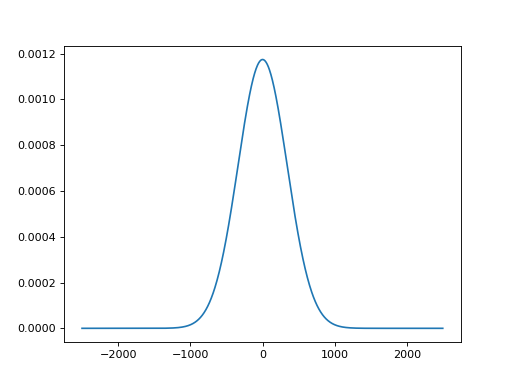

set_pulse_frequencies(omegas: Any) → None[source]#

Sets pulse frequencies

Parameters:: omegas (array of floats) – Frequencies of pulses

Examples

>>> lab = LabSetup()
>>> lab.set_pulse_frequencies([1.0, 2.0, 1.0])
>>> print(lab.omega)
[ 1.  2.  1.]

Situation which throws an exception

>>> lab = LabSetup()
>>> lab.set_pulse_frequencies([1.0, 2.0, 1.0, 6.0])
Traceback (most recent call last):
    ...
quantarhei.exceptions.QuantarheiError: Wrong number of frequencies: 3 required

get_pulse_frequency(k: int) → Any[source]#

Returns frequency of the pulse with index k

Parameters:: k (int) – Pulse index

Examples

>>> lab = LabSetup()
>>> lab.set_pulse_frequencies([1.0, 2.0, 1.0])
>>> print(lab.get_pulse_frequency(1))
2.0

set_pulse_arrival_times(times: Any) → None[source]#

Sets the arrival time (i.e. centers) of the pulses

Parameters:: times (array of floats) – Arrival times (centers) of the pulses

Examples

>>> lab = LabSetup()
>>> lab.set_pulse_arrival_times([1.0, 20.0, 100.0])
>>> print(lab.pulse_centers)
[1.0, 20.0, 100.0]

Situation which throws an exception

>>> lab = LabSetup()
>>> lab.set_pulse_arrival_times([1.0, 2.0, 1.0, 6.0])
Traceback (most recent call last):
    ...
quantarhei.exceptions.QuantarheiError: Wrong number of arrival times: 3 required

get_pulse_arrival_times() → Any[source]#

Returns frequency of the pulse with index k

Examples

>>> lab = LabSetup()
>>> lab.set_pulse_arrival_times([1.0, 20.0, 100.0])
>>> print(lab.get_pulse_arrival_times())
[1.0, 20.0, 100.0]

get_pulse_arrival_time(k: int) → Any[source]#

Returns frequency of the pulse with index k

Parameters:: k (int) – Pulse index

Examples

>>> lab = LabSetup()
>>> lab.set_pulse_arrival_times([1.0, 20.0, 100.0])
>>> print(lab.get_pulse_arrival_time(1))
20.0

set_pulse_phases(phases: Any) → None[source]#

Sets the phases of the individual pulses

Parameters:: phases (array of floats) – Phases of the pulses

Examples

>>> lab = LabSetup()
>>> lab.set_pulse_phases([1.0, 3.14, -1.0])
>>> print(lab.phases)
[1.0, 3.14, -1.0]

Situation which throws an exception

>>> lab = LabSetup()
>>> lab.set_pulse_phases([1.0, 2.0, 1.0, 6.0])
Traceback (most recent call last):
    ...
quantarhei.exceptions.QuantarheiError: Wrong number of phases: 3 required

get_pulse_phases() → Any[source]#

Returns frequency of the pulse with index k

Examples

>>> lab = LabSetup()
>>> lab.set_pulse_phases([1.0, 3.14, -1.0])
>>> print(lab.get_pulse_phases())
[1.0, 3.14, -1.0]

get_pulse_phase(k: int) → Any[source]#

Returns frequency of the pulse with index k

Parameters:: k (int) – Pulse index

Examples

>>> lab = LabSetup()
>>> lab.set_pulse_phases([1.0, 3.14, -1.0])
>>> print(lab.get_pulse_phase(1))
3.14

get_labfield(k: int) → LabField[source]#

get_labfields() → list[Any][source]#: Retruns a list of EField objects for the lab’s pulses

set_rwa(om: float) → None[source]#

restore_rwa() → None[source]#

get_field(kk: Any = None, rwa_frequency: Any = None) → Any[source]#: Returns the total field of the lab or a single field

get_field_derivative() → Any[source]#: Returns the time derivative of the total field

class quantarhei.spectroscopy.labsetup.labsetup(nopulses: int = 3)[source]#

Bases: LabSetup

labsetup is just a different name for the class LabSetup.

All details about usage of the labsetup can be found in the documentation of the LabSetup

class quantarhei.spectroscopy.labsetup.LabField(labsetup: Any, k: int)[source]#

Bases: object

Electric field of a single laser pulse defined within a LabSetup.

Objects of this class are linked to their parent LabSetup. Properties can be changed locally (affecting only this field) or globally from the LabSetup (affecting all linked LabField objects).

Parameters:

lab (LabSetup) – Parent laboratory setup object.
index (int) – Zero-based index of the pulse within the LabSetup.

Examples

Only the number of pulses has to be specified when LabSetup is created.

>>> lab = LabSetup(nopulses=3)

We can ask for a LabField object right away, even before field parameters are set.

>>> lf = LabField(lab, 1)

This object has all parameters “empty”

>>> lf.pol
array([ 0.,  0.,  0.])

>>> lf.om
0.0

>>> lf.tc
0.0

>> lf.phi 0.0

The ‘field’ property, however, refuses to return values

>>> print(lf.field)
Traceback (most recent call last):
    ...
quantarhei.exceptions.QuantarheiError: The property 'field' is not initialited.

Nor it can be set

>>> lf.field = 10.0
Traceback (most recent call last):
    ...
quantarhei.exceptions.QuantarheiError: The property 'field' is protected and cannot be set.

The LabField properties will be initialited through the LabSetup object. The only rule to follow is that arrival times of the pulses have to be specified before the pulse shape.

>>> lab.set_pulse_arrival_times([0.0, 0.0, 100.0])

>>> time = TimeAxis(-500.0, 1000, 1.0, atype="complete")
>>> pulse2 = dict(ptype="Gaussian", FWHM=150, amplitude=1.0)
>>> params = (pulse2, pulse2, pulse2)
>>> lab.set_pulse_shapes(time, params)

Everything else can be set before we ask for the field’s time dependence. The LabField object can be created even

>>> lab.set_pulse_polarizations(pulse_polarizations=(X,X,X),
...                             detection_polarization=X)
>>> lab.set_pulse_frequencies([1.0, 1.0, 1.0])
>>> lab.set_pulse_phases([0.0, 1.0, 0.0])

>>> lf = LabField(lab, 2)
>>> print(lf.get_phase() == lab.phases[2])
True

>>> lf.set_phase(3.14)
>>> print(lf.get_phase() == lab.phases[2])
True

>>> lab.phases[2] = 6.28
>>> print(lf.get_phase() == lab.phases[2])
True

>>> print(lf.get_center() == lab.pulse_centers[2])
True

>>> lf.set_center(12.0)
>>> print(lab.pulse_centers[2])
12.0

>>> print(lf.get_frequency() == lab.omega[2])
True

>>> lf.set_frequency(12.0)
>>> print(lab.omega[2])
12.0

>>> lf.get_polarization()
array([ 1.,  0.,  0.])

>>> lab.e[2,:] = [0.0, 1.0, 0.0]
>>> lf.get_polarization()
array([ 0.,  1.,  0.])

>>> lf.set_polarization([0.0, 0.0, 1.0])
>>> lab.e[2,:]
array([ 0.,  0.,  1.])

# we also have some quick access attributes

>>> print(lf.phi)
6.28

>>> lf.phi = 1.2
>>> lf.phi
1.2

>>> print(lf.phi == lab.phases[2])
True

>>> print(lf.tc)
12.0

>>> lf._center_changed
False

>>> lf.tc = 10.0
>>> lf.tc
10.0

>> lf._center_changed True

>>> print(lf.tc == lab.pulse_centers[2])
True

>>> print(lf.om)
12.0

>>> lf.om = 10.0
>>> lf.om
10.0

>>> print(lf.om == lab.omega[2])
True

>>> lf.pol
array([ 0.,  0.,  1.])

>>> lab.e[2,:] = [0.0, 1.0, 0.0]
>>> lf.pol
array([ 0.,  1.,  0.])

>>> lf.pol = [0.0, 0.0, 1.0]
>>> lab.e[2,:]
array([ 0.,  0.,  1.])

Most importantly, we can access the field values

>>> fld = lf.field
>>> fld.shape
(1000,)

and this property cannot be directly changed. >>> lf.field = 10.0 Traceback (most recent call last):

…

quantarhei.exceptions.QuantarheiError: The property ‘field’ is protected and cannot be set.

property phi: Any#

property delay_phi: Any#

property tc: Any#

property om: Any#

property pol: Any#

property field_p: Any#

property field_m: Any#

property field: Any#

get_phase() → Any[source]#: Returns the phase of the pulse

get_delay_phase() → Any[source]#: Returns the phase caused by the pulse delay

get_total_phase() → Any[source]#

set_phase(val: float) → None[source]#

Sets the phase of the pulse

Parameters:: val (float)

get_center() → Any[source]#: Returns the pulse center time

set_center(val: float) → None[source]#

Sets the pulse center time

val: float: The center of the pulse

set_delay_phase(val: float) → None[source]#: Calculate and set delay phases

get_frequency() → Any[source]#

set_frequency(val: float) → None[source]#

get_polarization() → Any[source]#

set_polarization(pol: Any) → None[source]#

get_fwhm() → Any[source]#

get_field(time: Any = None, sign: int = 1) → Any[source]#: Returns the electric field of the pulses

get_time_axis() → Any[source]#

set_rwa(om: float) → None[source]#

restore_rwa() → None[source]#

as_spline_function() → Any[source]#: Returns the spline represention of this field

get_pulse_envelop(tt: Any) → Any[source]#: Returns the envelop values

get_pulse_envelop_function() → Any[source]#: Return a function to be called later